Overview

The rainfall component of RWGEN uses a Neyman-Scott Rectangular Pulse (NSRP) model. Both single site (point) and spatial models can be configured in a standalone mode and as a component of a complete weather generator. This page provides an overview of the NSRP model concepts.

The rainfall model largely follows the earlier RainSim software described by Burton et al. (2008). For more detailed explanations of NSRP models see this paper and references therein.

Single Site Model

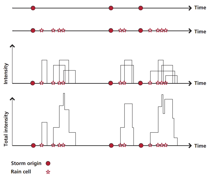
The basic single site (point) NSRP model consists of the following steps:

Begin by simulating storm origins

Each storm is then assigned a number of rain cells

Each rain cell is assigned an intensity and a duration

Total intensity at a moment in time comes from the sum of intensities of all active rain cells

This process is summarised in the diagram below (from Burton et al. (2008)). Each step is explained further below.

Storm Origins

Storm origins are simulated using a Poisson process, which is a model for a series of discrete events. The number of events (storms) in a time period is sampled from a Poisson distribution. Waiting times between events (storms) follow an exponential distribution.

A parameter λ (lambda) governs the rate of storm occurrence – i.e. number of storms (from Poisson distribution) and waiting times between storms (from exponential distribution).

Rain Cell Arrivals

Number of rain cells for a given storm is sampled from a Poisson distribution defined by parameter ν (nu). Arrival times of rain cells after the storm origin are then sampled from an exponential distribution using parameter β (beta).

Rain Cell Intensity and Duration

Each rain cell has a uniform rainfall rate throughout its lifetime. Rain cell duration and intensity are sampled from exponential distributions with parameters η (eta) and ξ (xi), respectively. However, other distributions can be used for intensity, e.g. Weibull, Gamma.

Final Rainfall Series

The total rainfall intensity at a moment in time comes from the sum of intensities of all active rain cells. As the NSRP process is continuous in time, it can be discretised into a time series with a desired time step (e.g. hourly, daily).

Parameters

The single site NSRP process described above requires a minimum of five parameters: λ (lambda), ν (nu), β (beta), η (eta) and ξ (xi). The parameters are typically also specified separately for each month of the year to account for seasonality (i.e. 12 x 5 parameters).

Parameters are identified by minimising the differences between a set of observed rainfall statistics and their NSRP model counterparts. The statistics include: mean, variance, skewness, autocorrelation and dry probability. Multiple durations can be used (e.g. 1- and 24-hour statistics) and statistics can be weighted differently. We need to use an optimisation algorithm to test different possible parameter values to arrive at the “best” ones.

Spatial Model

The single site NSRP can be generalised to simulate spatially consistent time series at any locations in a domain. The main difference in the spatial model is that rain cells (specifically cell centre locations) are simulated via a uniform spatial Poisson process. In contrast, the number of rain cells associated with a given storm is just sampled from a Poisson distribution in the single site model.

In the spatial model, the average number of rain cell centres in an area is prescribed via the parameter ρ (rho), although the exact placements of rain cell centres in a simulation exhibit randomness. Rain cells do not move in space in the model (i.e. no advection representation). A rain cell stays in the same location throughout its lifetime.

Each rain cell is assigned an arrival time, duration and intensity (uniform during cell lifetime) as per the single site model. In addition, each rain cell gets a radius sampled from an exponential distribution with parameter γ (gamma).

Total intensity at a point in space and time is the sum of intensities of all active rain cells.

Parameter fitting is as per the single site model, but also finding γ (gamma) and ρ (rho). Including spatial cross-correlations in the set of statistics used for fitting facilitates identification of these parameters.

Stationarity

It should also be noted that, before an additional adjustment, the spatial NSRP formulation is also spatially stationary in the statistical sense. This means that statistics (e.g. mean) are the same everywhere if averaged over a long period of simulation.

To have spatially varying statistics, we use a “scale factor” Φ (phi) proportional to the mean rainfall at a location to “rescale” the simulated time series. This scale factor can be calculated upfront from observations (and interpolated to ungauged locations if necessary). The mean and variance can now vary spatially, but other statistics (e.g. skewness, dry probability) cannot - at least in the basic spatial NSRP model.

Shuffling Method

The rainfall model has an optional, adapted implementation of the “shuffling” method proposed by Kim and Onof (2020). This method attempts to improve the performance of clustered point process rainfall models across timescales (from sub-hourly through to daily, monthly and beyond). This is achieved by nesting models and algorithms that work well at different timescales.

Three modules or layers are used in this nesting strategy:

Simulate a high (temporal) resolution series using the NSRP model

Shuffle storms using a similarity metric

Reorder months to match ranks of a coarse model (e.g. ARIMA)

The method and implementation is still undergoing evaluation, so it should be considered experimental at present.